第三講:Neural Processing and Perception
出自KMU Wiki
[編輯] Neural Processing and Perception
- 參照第52頁 封面
[編輯] Porcessing
- 參照第54頁 figure 3.1
[編輯] 複習Retina

- 結構
- rod/cone
- Amacrine cell
- horizontal cell
- bipolar cell
- ganglion cell

[編輯] Neural convergence
- 桿狀體如何作到較高的敏感度?
- 接桿狀體的節細胞,接受較多桿狀體的輸入
- 接錐狀體的節細胞,接受較少錐狀體的輸入
- 參照第43頁 figure 2.33
[編輯] Sensitivity vs Acuity
- Neural convergence 愈大敏感度愈高
- 只有好處嗎?
- 請看p.44 圖2.35
- trade-off
- 參照第44頁 figure 2.35
- trade-off sensitivity vs acuity
[編輯] Neural convergence...
- 資訊的聚集,就只為了增加敏感度?
- 請回憶上一章的
- p.43~44 圖2.32到2.35
[編輯] 鄰近接受器產生抑制作用

[編輯] 先從眼睛的演化來看
- Limulus (horseshoe crab,鱟)
- 參照第54頁 figure3.2
- 運作原理
- 參照第55頁 figure 2.3
[編輯] 從眼睛的演化來看

[編輯] lateral inhibition
- 側抑制
- 在神經系統常見的機制
- 目的:讓刺激更清楚(真有語病)
- 也造成「錯覺」
- Hermann grid(下圖)
- 參照第55頁 figure 3.4
[編輯] Hermann grid的可能原理交點上
- 參照第55頁 figure 3.5
- 參照第56頁 figure 3.6
[編輯] Hermann grid 在非交點
- 參照第56頁 figure 3.7
- 參照第56頁 figure 3.8
[編輯] 另一種側抑制錯覺Mach band
- 參照第57頁 figure 3.9
- 參照第57頁 figure 3.10
[編輯] Mach band可能原理
- 參照第57頁 figure 3.11
- 參照第58頁 figure 3.12
- 參照第58頁 figure 3.13
[編輯] Simultaneous contrast
- 參照第58頁 figure 3.14
[編輯] Simultaneous contrast可能原理
- 參照第59頁 figure 3.15
[編輯] A的灰與B的灰是一樣的!
- 參照第59頁 figure 3.16
[編輯] 不信遮一下
- 參照第59頁 figure 3.17
[編輯] 這不能用側仰制!
- 參照第60頁 figure 3.18
[編輯] 補充議題
- 演化與人類網膜
- fovea
- 接受器的分佈
[編輯] Fovea


- Fovea 中的接受器
[[Image:03Fovea3.png]
- 不同區域的分佈

- 離開網膜
- 由視神經離開
- 離開網膜
- 參照第60頁 figure 3.19
[編輯] 最初的接受區(receptive field)
- Hartline (1938) 青蛙實驗
- 參照第61頁 figure 3.20
[編輯] Harvard Medical School
- Kuffer (1953)在貓的retinal ganglion cell
- 參照第61頁 figure 3.21
- Kuffer測量
- 參照第62頁 figure 3.22
- 可能解釋
- 參照第62頁 figure 3.23
- Kuffer實驗情況
- 參照第63頁 figure 3.24
[編輯] processing 要進入腦中!
- 由Optic nerve 經 Optic chiasm (Optic tract )
- 到 superior colliculus
- 到 lateral geniculate nucleus
- 參照第63頁 figure 3.25
[編輯] Optic Nerve
- Optic Nerve(視神經)
- Optic chiasm(視交叉)
- Optic tracts(視束)
- Nerve -> chiasm -> tracts
- 其實都是retina ganglion cells的axon
- 解剖上的不同
- 其實都是retina ganglion cells的axon
- lateral projection(側投射)
- 不是左眼到右腦
- ipsilateral fibers(同側纖維)
- contralateral fibers (異側纖維)
[編輯] Superior colliculus(上丘)
- location
- top of brain stem(腦幹)
- function
- Multimodal(多感道) input
- control eye movement
- receptive field property(特性)
- lose center surround
- Phylogenetic(系統發生) – old
- Visual center for lower animals
- Frog, fish....
- In higher animals
- Superior colliculus的工作被visual cortex所取代
- 仍有的工作:Visual orienting
- 有receptive fields—but ill-defined ON OFF
- 對stimulus之where反應,what較不反應
- 結果—guidance of eye movement
- Multisensory cells(多重感覺細胞)
- Visual center for lower animals

- a.LGN接受來自丘腦(thalamus;T)和其他LGN神經元(L)的訊號,興奮性突處說明L,抑制性突處則是T,b.訊息經由LGN流入或流出,箭頭大小代表訊號大小
- 參照第64頁 figure 3.26
- LGN分六層,紅色層接收來自同側的訊號,藍色層接受來自對側的訊號
[編輯] Lateral Geniculate Nucleus

- Geniculate
- with bent knee
- magnocelluar layers
- parvocelluar layers

- 杯上點A.B.C在視網膜形成A.B.C影像,也在側膝核(LGN)活化A.B.C,這個在LGN和視網膜相同的圖象說明LGN有視網膜的圖像

[編輯] Maps in LGN

- retinotopic map

- retinotopic maps 中記錄的情況
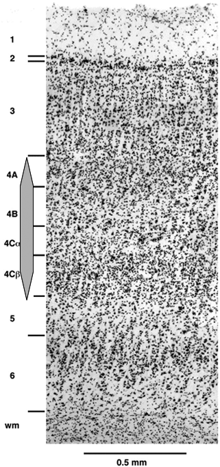
[編輯] Structure of visual cortex
- Primary visual cortex
- V1
- Area 17
- Striate cortex
- 1.5~2.0mm thick
- 100million cells in V1 each hemisphere
- 6 layers
- Layer 4 input from LGN

[編輯] Retinal map
- Topographic
- 80% cells 處理 10%的visual field
- 因此在視野中心的東西在cortical level放大很大
- 週邊視野的東西則變小
- 80% cells 處理 10%的visual field
- Contralateral(對側) visual field
- 以visual field來分lateral projection
- Contralateral(對側) visual field
[編輯] Receptive Fields of the Striate Cortex
- Hubel and Wiesel 的1950年代末到1970中一連串的研究
- Hubel and Wiesel 1981年獲得Nobel prize
- The Nobel Prize in Physiology or Medicine 1981
- Receptive Fields的形式
- orientation
- simple cortical cells
- 參照第65頁 figure 3.27
[編輯] Hubel and Wiesel當初發現的示意圖
- 參照第65頁 figure 3.28
- 參照第66頁 figure 3.29
[編輯] 到此的Receptive Field的特性
- Retina Ganglion cell-> Center-surround
- LGN -> Center-surround
- Simple cortical -> bar with orientation
- Complex cortical -> direction of movement
- End-stopped cortical -> length of movement bar
- 參照第67頁 figure 3.30
[編輯] Grating sti./ Contrast threshold
- 參照第67頁 figure 3.32
[編輯] Selective adaptation
- 知覺研究者的微小電極
- 原理
- 感覺神經如果有特異性(即針對特定的刺激才反應)
- 則長時間給于該刺激,則這個神經會疲勞(fatigue)
- 感覺神經疲勞,則其敏感度會下降,即絕對閾上升
- 所以如果有刺激可以在長時間曝露下,讓我們對該刺激的絕對閾上升,可以推論我們內在感覺神經系統對該刺激有「特異性」。
[編輯] 圖3.31 p.67之說明
- 參照第67頁 figure 3.31
- a. 先測量不同傾斜Grating偵測之threshold(是明暗對比的絕對閾,在閾限之下看起來是一片灰色)
- b. 曝露於高對比的Grating中(adaptation,適應過程)
- c. 適應之後,再量不同傾斜Grating偵測之threshold
[編輯] Selective adaptation之結果
- 參照第68頁 figure 3.33
[編輯] Selective Rearing
- 選擇性飼養
- 在特定(即只有限定品質)之環境下飼養動物
- 目的在於測試環境對於動物影響
- 初生動物之感覺剥奪是最常用的
- 本例為:Blakemore and Cooper (1970)
- 參照第69頁 figure 3.39
[編輯] Higher-level neuron
- 在更高層
- Inferotemporal (IT) cortex
- fusiform face area (FFA)
- Gross et al. (1972)
- 參照第70頁 figure 3.36
[編輯] IT and FFA
- 參照第69頁 figure 3.35
- Specificity coding
- 參照第70頁 figure 3.37
- Distributed coding
- 參照第71頁 figure 3.38
- Sparse coding
- 參照第71頁 figure 3.39
[編輯] Sensory coding
- 實際編碼方式(表徵 representation )
- Specificity coding (專一編碼)
- Distributed coding (分散編碼)
- Sparse coding (稀疏編碼 或 折中編碼)
- 實際可能
[編輯] 腦開刀時的測驗
- Quiroga et al., 2008
- 對於癲癎病人開刀(意識清醒下的開腦手術)
- 發現一個細胞專間針對
- Steve Carell(史提夫·卡爾) 反應
- 對於癲癎病人開刀(意識清醒下的開腦手術)
- 參照第72頁 figure 3.40
[編輯] The Mind-body problem
- Neural correlate of consciousness (NCC)
- easy problem of consciousness
- hard problem of consciousness
- 參照第73頁 figure 3.41
- 返回知覺心理學
